Four methods to find descriptive statistics by groups:

Descriptive statistics is the first encounter with the data, and gives us a primal intuition and idea of what is laid in front of us.

Sometimes, for some reason, we’re interested not only in the overall descriptive statistics of the whole sample, but in certain groups drawn from the sample.

There are several ways to achieve that:

First – let’s generate the data:

It’ll be the same data we’re using with a set.seed() function with the argument 1000.

This is the relevant code:

set.seed(1000)
Gender <- sample(size = 1000, replace = T, x = c("Male", "Female"))
City <- sample(size = 1000, replace = T, 
               x = c("NY", "LA", "Boston", "Chicago", "Denver", "London", "Paris", "Rome"))
Fav_Pet <- sample(size = 1000, replace = T, 
                  x = c("Cat", "Dog", "Fish", "Squirl"))

Salary_yearly <- sample(x = seq(55000, 150000), size = 1000, replace = T)
Weight_kg <- ifelse(Gender == "Male", sample(x = seq(80,120), size = 1000, replace = T), 
                    sample(x = seq(45,70), size = 1000, replace = T))  
Height_m <- ifelse(Gender == "Male", sample(x = seq(175,210), size = 1000, replace = T) / 100, 
                   sample(x = seq(155,180), size = 1000, replace = T) / 100)  

data <- data.frame(Gender, City, Fav_Pet, Height_m, Weight_kg, Salary_yearly)

Now that we have the data, let’s review the methods we can drill down and get further descriptive statistics for specific parts of the sample:

Method 1:

Using the summarize() function (from dplyr):

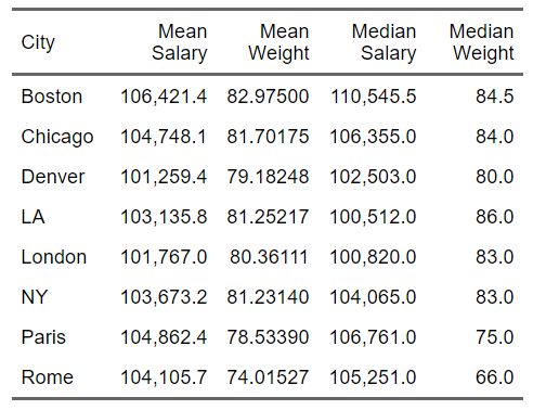
In this example, we’re interested in breaking the result by city, and we’re interested in means and the medians of the yearly salary, and weight in kg, but we can also use other measures like standard deviation, mode, variance and so on, and also go even deeper, and get even deeper descriptive statistics combining more than one splitting variable.

There’s the code:

# Method 1
data %>%
  group_by(City) %>% summarise("Mean Salary"=mean(Salary_yearly), 
                               "Mean Weight"=mean(Weight_kg), 
                               "Median Salary"=median(Salary_yearly), 
                               "Median Weight"=median(Weight_kg)) %>% flextable()

And there’s the result:

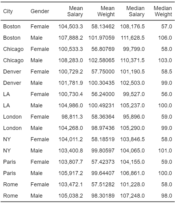
To see the combined descriptive statistics of both City and Gender, this is the relevant code:

data %>%
  group_by(City, Gender) %>% summarise("Mean Salary"=mean(Salary_yearly), 
                                       "Mean Weight"=mean(Weight_kg), 
                                       "Median Salary"=median(Salary_yearly), 
                                       "Median Weight"=median(Weight_kg)) %>% flextable()

And this is the following results:

Method 2:

Using tapply() function (from purrr package):

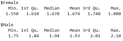
In this case, we’ll find the relevant measures of descriptive statistics of height in meters, by gender.

With tapply(), only one level of descriptive statistics is possible, unlike summarize().

This is the code for the result:

library(purrr)
tapply(data$Height_m, data$Gender, summary)

And this is the result:

Method 3:

Using split()  function (from Base-R):

This is quite similar to tapply() function, with ability to use only one level.

In this case, the analysis is relevant for all the variables in the data file, and not just one variable.

This is the code for that:

split(data, Gender) %>% map(summary)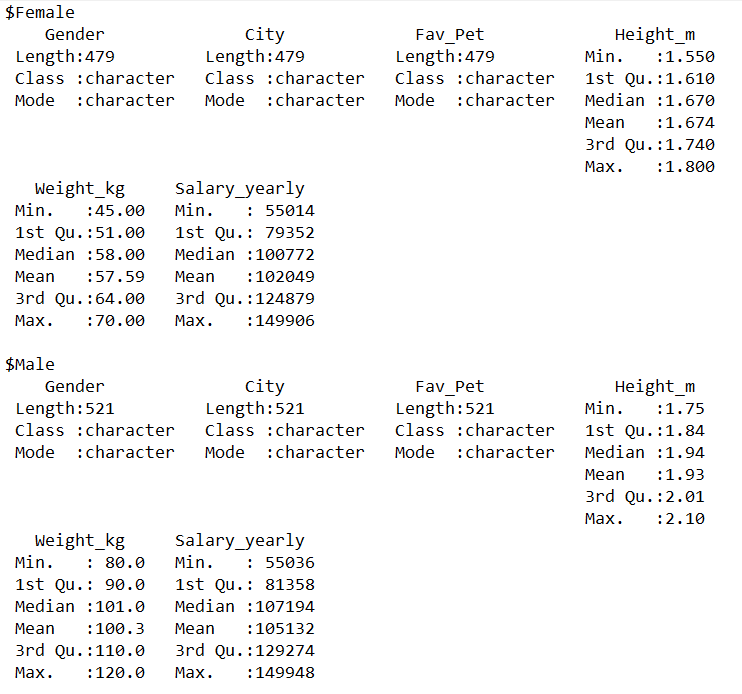

Method 4:

Using describeBy() function (from psych package):

In this case too, it’s impossible to drill down more than one level, but one can have information about a specific variable, or all the variables in the dataset.

This is the code for that:

library(psych)
describeBy(data$Height_m, group = c(Fav_Pet))

And this is the result: